The Yield Trap That Wasn't: Does Cheap-Market Cash Flow Really Erode Over the Hold?
An experienced investor recently pushed back on a piece I’d published — and the pushback was sharper than the piece. The misconception that actually costs investors money, he argued, isn’t about where yield is highest. It’s that the cash flow you underwrite on closing day is rarely the cash flow you keep. Initial cash flow flatters. Cheap, high-yield markets, he said, tend to cash-flow worse over a long hold than the spreadsheet promised — the opposite of what the day-one number leads you to believe.
It’s a widely held view, and a reasonable one. I went in expecting to confirm it. I couldn’t — and the reason it fails is more useful than the belief itself.
How to read this
Two ideas anchor everything below.
Initial yield is annual rent over purchase price on the day you buy: knowable, clean, and what every deal calculator shows you. Realized yield is what you actually earn across the hold, and it answers to things closing day can’t see — how fast rent grows, how much of that growth costs eat, and whether rent ever simply falls. Your mortgage is fixed; rent is the variable. So the durability of cash flow rides on the trajectory of rent, not its starting level.
The testable version of the belief: the markets with the highest initial yield — the cheap ones — should show the slowest subsequent rent growth, the starting advantage quietly bleeding away.
So I built it cleanly and went looking for the bleed.
The test
For 171 metros with enough liquidity to trust — active for-sale listings of at least 1,000, which filters out thin rural markets whose numbers swing on a handful of homes — I computed each metro’s entry yield as of April 2021: annualized rent over home value at the start of the hold, not a present-day stand-in. I sorted the 171 into five tiers by that entry yield, then measured how rents actually grew in each tier over the following five years. Then I re-ran the whole thing at four-year and seven-year horizons, so the result wouldn’t be a prisoner of a single start date.
If the erosion belief were right, the top tier’s rent-growth curve should bend downward. Here is what it did instead.
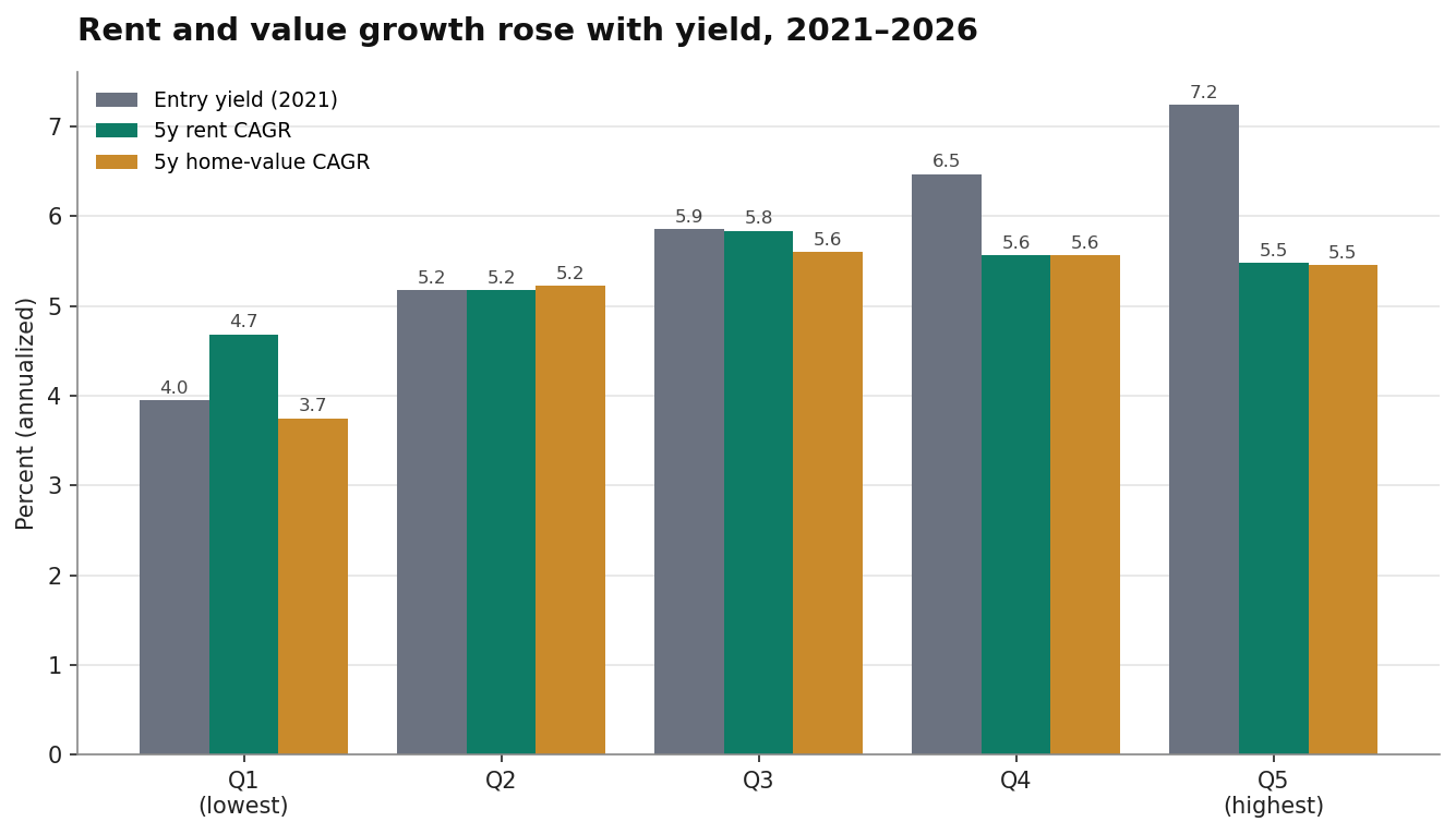
| Entry-yield tier | Median entry yield | n | 5y rent CAGR | 5y home-value CAGR | Exit yield (2026) |
|---|---|---|---|---|---|
| Q1 (lowest) | 3.95% | 35 | 4.68% | 3.75% | 4.12% |
| Q2 | 5.17% | 34 | 5.18% | 5.22% | 5.24% |
| Q3 | 5.86% | 34 | 5.84% | 5.60% | 5.88% |
| Q4 | 6.47% | 34 | 5.56% | 5.57% | 6.38% |
| Q5 (highest) | 7.24% | 34 | 5.48% | 5.45% | 7.40% |
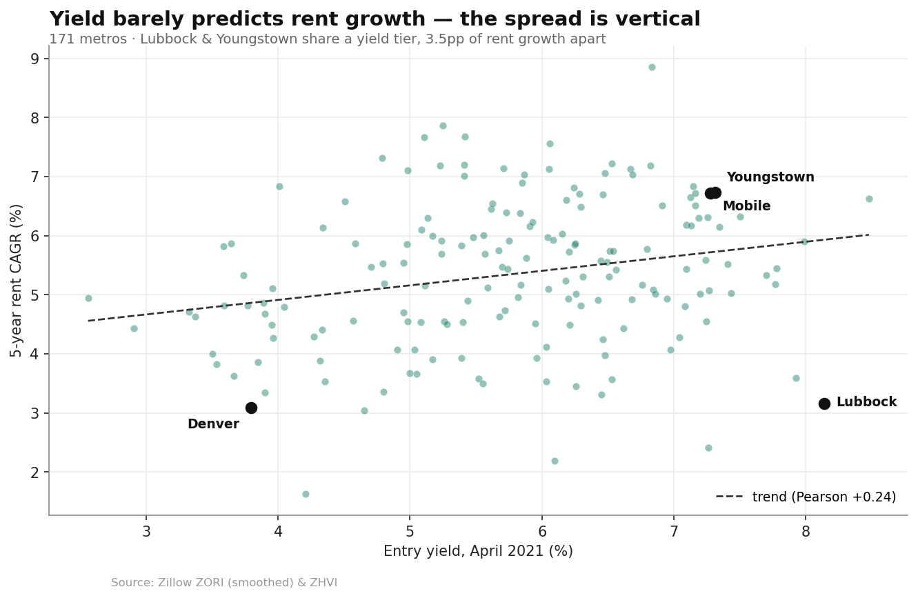
The relationship runs the wrong way for the erosion thesis. Rent growth rises from the lowest-yield tier through the middle, then plateaus — it does not collapse at the top. The lowest-yield tier grew rents a median 4.68% a year; the highest-yield tier grew them 5.48%. The correlation between entry yield and rent growth is positive — Pearson +0.238 — the opposite sign from what the belief predicts.
And it held across every window. At four years the correlation was +0.247, at five +0.250, at seven +0.245 — parked in the same narrow band no matter where the hold was anchored. If anything, the five-year window is the kindest framing the erosion belief ever gets: its top-to-bottom gap is the smallest of the three. The four-year window — the most recent stretch, when coastal demand was supposed to be reasserting after the pandemic — is the most damaging to it: the highest-yield metros grew rents 4.06% a year against the lowest tier’s 2.30%, nearly double. The start date most favorable to the belief still refuses to support it.
A natural objection: tiering by today’s yield could bias the result, since current yield and recent rent growth share a term. They don’t drive it. Tiering strictly by April-2021 entry yield — independent of subsequent rent growth — gives the same answer, and 77% of metros land in the same quintile under both definitions.
The effect is real — and small
Honesty about size matters here, because the headline is louder than the effect.
A correlation of +0.24 explains about 6% of the variation in rent growth. Entry yield nudges the odds; it determines nothing. The real action isn’t between the tiers — it’s inside them.
Take the top yield tier, the “cheap markets” at the center of the belief. Split it open and it is bimodal. The Texas and oil-economy metros stagnated, exactly as the erosion view would predict — Lubbock grew rents 3.16% a year, McAllen 3.59%, Corpus Christi a tier-worst 2.42%. But the Rust Belt and Deep South metros sitting in the same yield band did the opposite — Youngstown 6.73%, Mobile 6.72%, Montgomery 6.33%, Rochester 6.15%.
Same entry-yield band. Same five years. Lubbock and Youngstown started at effectively the same yield and finished three and a half points of annual rent growth apart. The erosion pattern is real — but it is a Texas-and-oil pattern, not a cheap-market pattern. Yield tier did not sort the winners from the losers. The local economy did.
That turns the finding into something more useful than a refutation. Yield tier is a weak signal. The economy underneath it is the strong one. Buy the yield while ignoring the sub-economy, and you might catch Lubbock thinking you had bought Youngstown — identical on the day-one number, four points apart over the hold.
The part that should give a coastal investor pause
There is a second number in that table that quietly does more damage to conventional wisdom than the rent-growth column.
The standard defense of low-yield coastal and Mountain-West markets is that you trade current cash flow for appreciation — and, eventually, for cap-rate compression that lifts your exit value. Over this hold, on these numbers, that trade lost on every leg.
Start with compression: it didn’t happen, on either end. The lowest-yield tier entered at a median 3.95% and exited at 4.12%; the highest entered at 7.24% and exited at 7.40%. Both drifted slightly up. Nobody on either side was bailed out by falling cap rates.
Then appreciation — the whole reason to accept a low yield. The high-yield tier appreciated faster: median home-value growth of 5.45% a year against 3.75% in the low-yield tier, a 1.7-point annual gap, compounding. The cash-flow markets out-appreciated the appreciation markets.
Denver makes it concrete. A Q1 favorite, it grew rents 0.58% a year over the most recent four and appreciated 2.35% a year over five. Mobile, Alabama — three-plus points higher on entry yield — grew rents 6.72% and appreciated 4.71%. That is not supposed to happen if yield and growth trade off against each other. Over this particular five years, the high-yield metros won rent growth, won appreciation, and kept their yield. A clean sweep.
The fences
A finding this tidy needs them.
This was one specific hold, and a distinctive one: the 2021–2026 migration wave that pulled people and capital into Sun Belt and Rust Belt metros and away from the expensive coasts. The high-yield tier’s clean sweep reflects that regime. It is not a law of real estate. Run the same test across 2006–2011 and the answer would look different — which is, in fact, the deepest point the investor raised, and the one this data does not touch. He argued that cash flow is never certain, that rents can fall outright, as they did across Detroit, Phoenix, and Las Vegas after 2008. This window contained no national rent recession, so it has nothing to say about that risk. The erosion-as-a-rule claim does not survive the data. The rents-can-fall claim was never in the sample to test, and it is real.
And the effect is modest. A +0.24 tilt is a lean, not a law. If you take one number from this, don’t let it be the correlation — let it be the dispersion. The spread within any yield tier dwarfs the gap between tiers, every time.
What this means
Initial yield is a weak predictor of the yield you keep — but not in the direction the conventional wisdom claims. It doesn’t reliably erode, and it doesn’t reliably compound. Mostly, it just doesn’t tell you much. What tells you something is the engine underneath the number: the local economy growing or stalling the rent that turns a closing-day figure into a five-year reality. That is the variable worth your attention, and it is invisible on the day-one spreadsheet.
It is also, not coincidentally, the thing market-level demand and stability data is built to surface — the same engine behind the Investor Market Scorecard, which ranks markets on growth and stability rather than yield alone.
With thanks to Dan, whose pushback is the reason this analysis exists. He may not love where the data landed, but he asked the right question — and the right question is worth more than a comfortable answer.
Method
Universe. 171 metros with at least 1,000 active for-sale listings, the noise floor below which thin markets distort the extremes. Sufficient rent history exists for 718 metros; the liquidity floor reduces the set to 171. Lowering it to 500 does not change the tier signal.
Entry yield. Annualized April-2021 rent over April-2021 home value, per metro, ranked into quintiles. Rent uses the smoothed, seasonally adjusted rent index; home value uses the standard home-value index. A proxy tiering on current yield places 77% of metros in the same quintile, so the choice of definition does not drive the result.
Growth. Compound annual growth rate, end over start, across three windows: four years (Apr 2022→2026), five years (Apr 2021→2026), and seven years (Apr 2019→2026). Reported figures are tier medians.
Correlation. Entry yield vs. 5-year rent CAGR: Pearson +0.238, Spearman +0.248. Entry yield vs. 5-year home-value CAGR: Pearson +0.290, Spearman +0.272.
Caveat. All figures describe a single 2021–2026 hold, a period of unusually strong Sun Belt and Rust Belt in-migration. The window contains no national rent decline, and the results should not be read as regime-independent. Data: Zillow ZORI (smoothed) and ZHVI.